JS Optimization Documentation
Background
Originally this repository was part of a project for the course "Optimization
Methods for Engineers" (227-0707-00L) at ETH Zurich.
The goal of the project was to
implement an optimizer for a chosen problem and write a report about the results.
Documentation Credit
This documentation uses styles and JavaScript taken from the Google Style Guides (with minor changes).
Project Goal
This repository implements multiple optimizers for the Job Shop scheduling problem. Among the many variations of the problem the following definition is used:
An instances of the Job Shop scheduling problem consists of N Jobs that need to be
scheduled on M machines. Each Job in turn consist of Tasks that have
a processing order. Each of the Jn Tasks of Job n has their own processing
time and machine requirement.
A machine can only process a single Task at a time and
processing is not preemptable.
For a rigorous description please consult this excerpt from the report, which gives the mathematical problem definition.
Additionally the repository contains infrastructure to deal with:
- Problems,
- Solutions,
- and Search Space Representations.
Components Overview
The JS_Optimization Visual Studio Solution contains three projects. They are two libraries (JS_Lib and Loguru) and the entry point JS_Optimizer.
The following subsections briefly describe each project.
JS_Optimizer
This project is designated as the executable for the CMake build and contains the main.cpp file.
The JS_Optimizer project servers as a minimal wrapper for the JS_Lib functionality
and enables the creation of actual executables that perform optimization.
There is no proper user interface, the configuration of the optimizations is done by
changing the code in the main.cpp file.
Besides the main function it contains the following functions:
- a small sanity test function to verify that the project is setup correctly
- a bigger test that exercises all the functionality
- the 'runOptimizer' template function that shows how to create a Problem and Optimizer and then run the Optimizer. It also shows how to validate and store the Solution. The configuration needs to be done manually.
- the 'evaluateOptimizers' function that uses the StatsCollector utility class to run and log an Optimizer on problems in bulk.
These functions and the comments in the main function should provide ample usage examples.
Some global variables that define the default absolute file paths are automatically setup with the CMake build. The absolute paths are expected by the Problem and Solution constructors.
JS_Lib
This project is the core functionality. All the optimization code is completely
contained inside the JS_Lib project.
To use JS_Lib include
'JS_Optimization/JS_Lib/include/JS_Lib.h' in your project.
The code in JS_Lib can be grouped like this: problem_base, optimizer_base, optimizers and utility.

The 'problem_base' enables the creation, saving and loading of Problem instances. It also defines the general Solution object that all optimizers ultimately generate. The Solution class enables saving and loading of solutions and it also offers a solution validation utility.
The 'optimizer_base' code defines 'Optimizer.h', a base class for all optimizers.
It also defines multiple possible representations on which an optimizer can operate.
The representations provide initialisation and basic manipulation of the representation
as well as the creation of Solutions from the internal state.
Optimizers choose a representation and then define the initialisation, iteration and termination functions for the optimization process of the optimizer. Currently there are four different optimizers implemented.
Both new representations and optimizers can be added.
All optimizers should subclass/extend the Optimizer class defined in Optimizer.h.
However using a representation is not required.
For more details see the JS Lib section below.
All the different header files are directly accessible without the need to specify the path through the subfolders in the source tree. Since this is a small project I choose convenience over the more principled approach. If many additional files are to be added, I would recommended using subfolders inside the current folders. With the current CMake configuration, these folders should not be added to the include path automatically. This should limit the issues that arise from the extended include path.
Loguru
The logging needs of the project are covered with "Loguru" by emilk. See his GitHub repository.
Version 2.1.0 cloned in April 2023 is included/setup in this repository. Refer to it's documentation and the README in the JS_Optimization/loguru/ folder for usage details.
To use it simply include the 'loguru.hpp' header. CMake is setup such that direct inclusion without any path prefix is possible.
Dependencies
The project uses CMake to setup the Visual Studio solution, hence it requires both CMake and Visual Studio. C++20 is required to compile the source code.
There are a couple optional helper scripts that require a Python installation
(see Python Helper Scripts).
Some of the scripts use
Google OR-Tools.
They require the installation of the 'ortools' package, see the
Installation Guide
from the Google OR-Tools website.
JS_Lib
The following sections will cover the JS_Lib components in more detail. But this documentation does not aim to provide a User Manual for the code. The usage of the code should be evident from the names and the comments.
Instead the conceptual ideas behind the components will be explained. Additionally what functionality each component offers will be covered.
Problems
Problem objects can be created from text files. The constructor requires the path and name of a file (including the file extension) that contains a valid problem description. There are two separate formats for the layout inside the text files, see Problem Description, which format is used must also be supplied to the constructor.
A problem instance is immutable but provides a number of constant getter functions to inspect it's contents.
An invalid file or file content will abort execution.
Each Problem also has a Problem::Bounds instance associated with it. The Bounds object provides some absolute lower bounds on the completion time of the Problem.
The Problem class offers:
- Loading of Problem instances from files in both file formats (using absolute paths).
- Creation of Problem instances from a given Solution.
- Saving of Problem instances to a file (with a format selection).
- Accessor methods to inspect a Problem.
- Basic timing bounds information about the Problem with the Problem::Bounds class.
See Problem.h for the details.
Problems should be in saved in the 'JS_Optimization/JobShopProblems/' folder. The 'JS_Optimization/JobShopProblems/Instances' should not be renamed, as
Solutions
Solution instances usually get created by Optimizers. Typically the Representation the Optimizer uses implements a nested class that extends Solution and provides a constructor for Solutions.
Solutions are immutable. They are shared between the user code and the Optimizer itself. This is done safely with std::shared_ptr.
Solutions have their own file format (see Solution Description). This format contains quite a lot of redundancy, this is used for faster and more thorough integrity checking and prevents the validation from inferring incorrect parameters.
Since the Solution class contains redundancy and is immutable it should not be used to store the internal solution state of optimizers. Instead a SolutionConstructor that subclasses Solution should be implemented. SolutionConstructor then converts the internal solution state to a canonical Solution. Since the internal solution state should only change between Search Space Representation and not between Optimizers on the same Representation, each one should supply the SolutionConstructor.
The Solution class offers:
- Loading of Solutions from files (using absolute paths).
- Saving of Solutions to files (and by extension Visualization with the Python scripts), using absolute paths.
- Accessor methods to inspect basic properties like the makespan, task count, etc.
- The Solution validation to check if a Solution is valid with respect to a given Problem instance.
- A view of the Tasks in Problem order
See Solution.h for the details.
Optimizer Base
Optimizer_base contains Optimizer.h which is the base class for all optimizers. Having a base class allows easy polymorphism and gives all optimizers a unified interface.
The other classes in 'JS_Optimization/JS_Lib/optimizer_base/' implement Search Space Representations. They subclass the Optimizer base class.
Optimizer.h
Optimizer.h is an Abstract Class and defines some pure virtual functions, that need to be implemented by each optimizer. They are:
void Initialize()
initializes an optimization run
void Iterate()
performs an optimization iteration
bool CheckTermination() const
returns true if the termination criteria are reached
std::shared_ptr<Solution> getBestSolution()
get current best solution, sharing ownership
std::string getOptimizerName() const
allows easy identification if used with polymorphism
Optimizer.h also contains a 'Run' function with a default implementation that can be overridden.
Typically an optimizer subclasses an Representation. It provides implementations for the functions mentioned above and uses the utilities the Representation provides.
The Representations that are provided in JS_Lib are described in their own sections below.
Optimizer Base also defines the Termination Criteria struct with the three different criteria: total iterations, restart count and a percentage relative to the lower bound. The 'CheckTermination()' should use this. Since the concept of an iteration may vary for different optimizers there is no default implementation for it.
Search Space Representations
The Representations are part of Optimizer_base. All of them subclass Optimizer.h. But they do not implement the pure virtual functions of Optimizer.h since they are intended to function as support for the actual Optimizers.
The following sections will discuss all the Representations.
Index
Machine Order representation
This Search Space Representation is straight forward. All Tasks are grouped per machine and placed in multisets. Then Tasks are pulled from a set to build the precedence order for the machine the set corresponds to.

The schedule uses indirection to prevent a Task from Job x getting scheduled before another Task from Job x on the Machine that has a lower index. Meaning that the Set of Tasks is actually represented as a multiset of Job ids. The clique has an ordered list of task ids for each job. By tracking how far along the list each Job is, it is guaranteed that each Machine has an internal precedence order that is valid.
This only covers half the conflicts that may occur. The solution may still be unfeasible due to deadlocks across multiple machines. This is the major downside to this representation. It is very difficult to find and resolve these conflicts in this representation. The solution constructor will return uninitialized solutions should the current state be invalid. In that case the Solution will have a 'makespan_' of -1 and the 'initialized_' bool will be false.
Each Machine has an instance of the MachineClique class which provides some getters and the current schedule for the machine. The schedule can be retrieved with the 'getMachineOrder()'. It's contents should remain the same, only the order may be modified, else the Solution will be invalid with respect to the Problem.
The representation builds the machine cliques and mappings. The initial state is the sequential Solution obtain by scheduling the Jobs in ascending order. It also provides a Solution Constructor that builds the Solution from the current state the cliques contain.
The specific optimizer only needs to decide how elements are reordered in the cliques.
Global Order representation
Like the name suggests, this Search Space Representation uses a global ordering. The core of the Representation is a list that contains each Job Task-count times. This indirection functions similarly to the Machine Order and is used to prevent deadlocks from occurring.

The Index Lookup informs us how far along the list in the Lookup Table we are. This ensures each Job is conflict free. The global order intrinsically prevents conflicts across different Machines.
For these reasons the Global Task Order representation is only able to represent valid solutions. It can also still represent all possible solutions. The trade off is that this Representation increases the size of the Search Space significantly. The reason being that the number of permutations of the Total Order list is significantly larger than the combined number of permutations of all the individual Machines.
In practice this is an acceptable trade off. The two main reasons for this are:
- the original search space is already too large to be searched by brute force
- the number of invalid solutions is far larger than the number of valid solutions
The Representation implements a constructor that creates an initial Total Order, representing the sequential solution. It also provides the SolutionConstructor that builds the Solution corresponding to the current Total Order.
The representation does not provide any utilities to provide information about bottlenecks in the schedule. An optimizer requiring such information has to implement this themselves. This is not provided for efficiency reasons, as the optimizer needs to decide very specifically what information it requires. Since the Representation loses a lot of information and it is expensive to recompute it.
Graph representation
The Disjunctive Graph Representation is well known in literature. It is rather complex but makes a lot of information easily accessible. It also enables targeted manipulation of the current schedule.
Each vertex in the graph represents a Task. There are two kinds of edges. The Rp relation contains edges that capture the immutable constraints of the problem instance (i.e. the Task processing order), also called the conjunctive arcs. The machine cliques are the mutable edges that an optimizer can change, also called the disjunctive arcs. They represent the actual schedule.
This is the initial state of the representation:

The machine cliques are groups of nodes that are connected by a complete graph of bidirectional edges (colour coded in the figure). They represent Tasks that need to be processed on the same Machine. For example the Tasks represented by vertices T10, T01 and T21 are one machine clique.
To create a schedule all the bidirectional edges need to be directed. The directed edges then define a schedule for the machine they belong to. The schedule is valid if and only if the complete graph containing both the Machine Clique edges and Rp edges is acyclic.
GraphRep initializes all the immutable edges in the graph but leaves it up to the optimizer to insert the mutable edges (usually done with DacExtender). The cliques_ member contains a list for each Machine that holds all the vertex ids that belong to the clique.
The GraphRep.h class provides a number of helpers to achieve this. The main ones are:
- PathsInfo
- DacExtender
- other helper functions
- Solution Constructor
Each PathsInfo instances are tightly coupled with a single GraphRep instance. PathsInfo calculates the Critical Path of the current graph/schedule. It does this with the critical path method (CPM). A notable by-product of CPM is the current makespan of the graph. The main output of the CPM is the list of vertices on the critical path, but the concrete timings are available for all vertices.
DacExtender is a dynamic topological sorter. It takes an acyclic graph as input and then provides the 'InsertEdge()' function which takes two vertices as arguments and returns a directed edge that maintains the acyclic property of the graph. DacExtender performs deterministic insertion of new edges. But by randomizing the insertion order, the result can be randomized. This enables deterministic time random generation of initial DAC's that an optimizer can iterate on (i.e. random restarts).
There are a few helper functions to facilitate the changing of the internal graph, see GraphRep.h. They include a reachability and a cycle checker.
The SolutionConstructor simply creates a Solution from the internal state.
It also has mappings from vertices to Tasks and a separate mapping to the duration of the Task directly to avoid a double lookup.
Sub-classing GraphRep
NOTE:
- If an optimizer manually changes the graph, it must set the 'modified_flag' bool member. If this is not done correctly PathsInfo will perform no-ops when update is called.
- Two additional special vertices are introduced when a problem is loaded. A source (id:0) and a sink vertex (id:vertex_count_-1).
- GraphRep uses unified successor and predecessor lists. Positive values encode successors and negative values predecessors. Additionally the immutable Rp edges are separated from the mutable Machine Clique edges. This is done by adding an offset of vertex_count_ to the Machine Clique edges before any other operations. Combined this means for each vertex all neighbours can be found by iterating over graph_[vertex_id] and they can easily be filtered for predecessor, successor and mutability.
Optimizers
All Optimizer's subclass one of the optimizer_base classes. The different Representation classes implement some common functionality that a given search space representation may need. See their header files in JS_Lib/optimizer_base/ or the Optimizer Base section of the documentation.
The optimizers themselves are not meant to be sub-classed.
All optimizers should subclass Optimizer.h. Either directly or indirectly through a representation. And consequently they must implement the pure virtual functions Optimizer.h defines (listed here).
The following sections will briefly describe the Optimizers that are already implemented.
RandomSearch Optimizer
This is a classic 'Random search' optimizer on the Total Order Representation.
It simply randomly shuffles the list containing the total order.
RandomSearchMachine Optimizer
This is a classic 'Random search' optimizer on the Machine Order Representation.
It randomly shuffles the list with the ordering of each machine.
RandomSwap Optimizer
This is a 'Simulated Annealing' optimizer on the Total Order Representation.
It has all the typical components of a Simulated Annealing optimizer:
- a temperature that starts high and decreases with time
- making more changes per iteration if the temperature is higher
- a chance to accept worse Solutions that decreases as the Temperature decreases
- early random restarts if no progress is made for a number of iterations
This optimizer uses a simple neighbourhood definition. Two solutions are direct neighbours if the schedule of one can be transformed into the other by performing a single swap of two consecutive elements in the total order list.
ShiftingBottleneck Optimizer
This is a 'Simulated Annealing' optimizer on the Graph Representation.
It has all the typical components of a Simulated Annealing optimizer:
- a temperature that starts high and decreases with time
- making more changes per iteration if the temperature is higher
- a chance to accept worse Solutions that decreases as the Temperature decreases
- early random restarts if no progress is made for a number of iterations
This optimizer uses a number of heuristics to preselect swaps to alter the critical path of the graph. The choice of which swaps to perform is randomized. The number of swaps is determined by the temperature. See this excerpt of the report for a more detailed description of the heuristics.
Performance Overview
ShiftingBottleneck is the best among the implemented optimizers. It is also by far the slowest. It can find decent solutions with 2000 iterations. With the release build this should not take more than a couple minutes on decent hardware, even for the largest problems in the Instance folder. But it tends to bottleneck itself due to the implemented heuristics stalling in local optima. Because of this increasing the iteration count is usually not beneficial. Instead using more seeds and doing more runs with them is the better option to find better solutions.
RandomSwap and RandomSearch are essentially equivalent. They use the same Representation and although RandomSwap uses a different approach it relies on a neighbourhood definition that does not contain useful information. Consequently its behaviour is equivalent to the random shuffling RandomSearch does. These two Optimizers are very fast and given enough time could find the optimum. However the search space is many times too large for even a supercomputer to evaluate a decent percentage of the search space. For a low number of iterations, say under 10'000, ShiftingBottleneck should outperform these two consistently.
RandomSearchMachine is basically useless. It usually fails to find valid solutions at all. It only has a chance for very small problems. The reason being that the cross machine conflicts are far too common, making a vast majority of the schedules invalid.
Utility
The classes in Utility are:
- Utility.h
- Heap.h
- StatsCollector.h
- Parser.h
- FileCollector.h
Utility.h has remove_at() and randomPullUniqueFromRange(), which may be useful for optimizers to access a container like a vector. The other two functions are helpers to deal with file paths.
The Heap class is a wrapper around the std::make_heap and friends of <algorithm> and can be both a Max or a Min heap based on the comparator. The original intent was to store multiple solutions in a max heap, but this idea was overturned in favour of std::shared_ptr's and the heap is no longer used anywhere.
StatsCollector is a simple template class that runs an Optimizer on multiple problems and logs the results in a csv file. It is very useful to test Optimizers in bulk. The class is configured with the default folders of the Solutions and Problems. This is not configurable with arguments since it would only add multiple arguments that would always be a default value, given the current setup. It is the only class that has such a dependencies to the environment. The locations can be changed easily by changing the const members should it be required. For usage examples see the comments in main.cpp and the evaluateOptimizers() function in particular.
Parsing.h is used by the Problem class to load instances from files.
FileCollector.h is used to collect the Problem files for StatsCollector.h. It only collects files in with the .txt file extension.
Adding new Optimizers
Things that should not be overlooked if you want to add an optimizer:
- do not forget to add the new Optimizer to JS_Lib/include/JS_Lib.h
- you need to implement the virtual functions of optimizer.h
- you probably should not use the Solution class to store the optimizer state, it contains way too much redundancy for that
- the search space you use is the most important decision, and using one that only contains valid solutions is a major help, otherwise you need to deal with the invalid schedules and that takes a lot of effort
- the Solution class has a protected method that is very useful for Representations, After the SolutionConstructor has correctly mapped the internal state into the new Solution, the CalculateTimings() function can determine all the start and end times.
Naming Conventions
The naming conventions mainly follow the Google Style Guide for C++. I focused on these rules:
- use the wider supported '#ifndef', '#define' guards instead of the '#pragma once' guard to prevent duplicate includes
- generally prefer long names over abbreviations, especially "custom" abbreviations
- types should capitalize each word i.e. 'ObjectName'
- all variables are in snake case i.e. 'some_variable'
- private class members end with a underscore i.e. 'member_variable_', struct members do not have this
- functions capitalize the start of all words i.e. 'FunctionName'
- getter functions and static functions do not capitalize the first word i.e. 'getCount'
File Formats
Problems and Solutions are stored and read from text files. There are three file formats, two for Problems and one for Solutions. The required formats are detailed in the next sections
Problem Description
A Job Shop problem consists of Jobs, a Jobs consists of Tasks, a single Task runs on a specific machine and takes a set amount of time.
This project supports two formats, called Standard and Detailed. For custom problems the Detailed format is recommended because it allows for more consistency checks during parsing.
The Standard format was introduced to be compatible with the format used for the public JobShop Instances that were/are researched and have known optima.
Detailed Format
To define a problem in the Detailed specification, follow:
- The first line contains two numbers: 'job count' and 'machine count', they specify how many jobs and how many machines the problem contains
- Every line afterwards defines exactly one Job. This is done by first specifying the number of Task the Job has. Then each Task is specified by a pair that defines the 'machine' and 'duration' of the Task. The sequence of the Tasks on a line defines the order in which the Tasks need to be processed.
- The comma separator between the pairs can be replaced by any character or omitted altogether (commas are recommended for readability).
- Both tabs and spaces are valid white-space characters. The parser also handles multiple white-spaces correctly.
For the Task definitions to be legal 'machine' has to be in the range [0,machine_count] and 'duration' must be >= 0. All values must be integers. The number of Jobs must also match the number of Jobs that was specified on the first line.
The file may begin with a comment block. The comment must be a continuous block of lines, each starting with '#'.
# comment lines are possible, no indentation allowed before '#'
3 5
6, 0 8, 3 6, 4 10, 0 3, 1 9, 2 5
4, 3 4, 0 12, 4 16, 3 8
7, 4 19, 2 8, 0 6, 1 10, 3 7, 1 5, 2 9
JobShopProblems/SmallTestingProblem.txt
Standard Format
To define a problem in the Standard specification, follow:
- The first line contains three numbers: 'job count' and 'machine count' and 'lower bound', they specify how many jobs and how many machines the problem contains as well as the known optimal lower bound (use -1 if the lower bound is unknown)
- Every line afterwards defines exactly one Job. This is done by giving a pair for each Task. The pair defines the 'machine' and 'duration' of the Task. The sequence of the Tasks on a line defines the order in which the Tasks need to be processed. Only white-space separators are allowed.
- Both tabs and spaces are valid white-space characters (the files from JobShop Instances use tabs).
For the Task definitions to be legal 'machine' has to be in the range [0,machine_count] and 'duration' must be >= 0. All values must be integers.
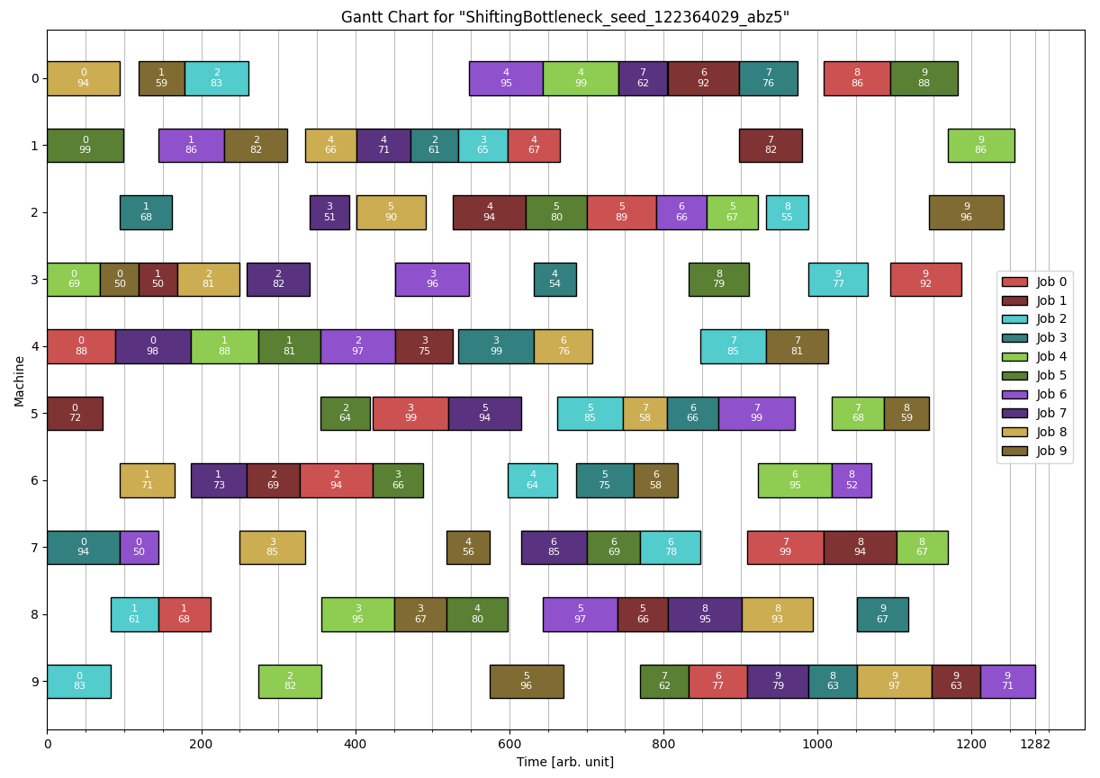
10	10	1234
4	88	8	68	6	94	5	99	1	67	2	89	9	77	7	99	0	86	3	92
5	72	3	50	6	69	4	75	2	94	8	66	0	92	1	82	7	94	9	63
9	83	8	61	0	83	1	65	6	64	5	85	7	78	4	85	2	55	3	77
7	94	2	68	1	61	4	99	3	54	6	75	5	66	0	76	9	63	8	67
3	69	4	88	9	82	8	95	0	99	2	67	6	95	5	68	7	67	1	86
1	99	4	81	5	64	6	66	8	80	2	80	7	69	9	62	3	79	0	88
7	50	1	86	4	97	3	96	0	95	8	97	2	66	5	99	6	52	9	71
4	98	6	73	3	82	2	51	1	71	5	94	7	85	0	62	8	95	9	79
0	94	6	71	3	81	7	85	1	66	2	90	4	76	5	58	8	93	9	97
3	50	0	59	1	82	8	67	7	56	9	96	6	58	4	81	5	59	2	96
JobShopProblems/Instances/abz/abz5.txt
The two relevant differences between the two formats are:
- Detailed format: specify number of Tasks (i.e. Pairs) at the start of each line
- Standard format: specify the lower bound of the problem on the first line
Solution Description
Solutions have one format. The Python visualizations scripts that create Gantt Charts depended on this to parse Solutions, in particular the comma separator is mandatory.
The format to define a problem in the Standard format is as follows:
- The first line is the name of the Solution. This is accessible if the Solution is loaded in the C++ program and it will be displayed in the Python visualizations.
- The second line contains two numbers: 'job count' and 'machine count', they specify how many jobs and how many machines the Solution contains
- Every line afterwards corresponds to a machine. The first number is the number of Tasks the Machine processes. After that there is a six-tuple for each Task. The tuples are separated by commas and have the format: 'job id' 'task index' 'machine' 'duration' 'start time' 'end time'
The Tasks and Jobs that can be reconstructed from the Solution must match the Problem it should solve. This can be checked with the Solution::validateSolution() function for arbitrary pairs of Solutions and Problems.
During parsing the first continuous block of lines starting with '#' will be ignored as comments.
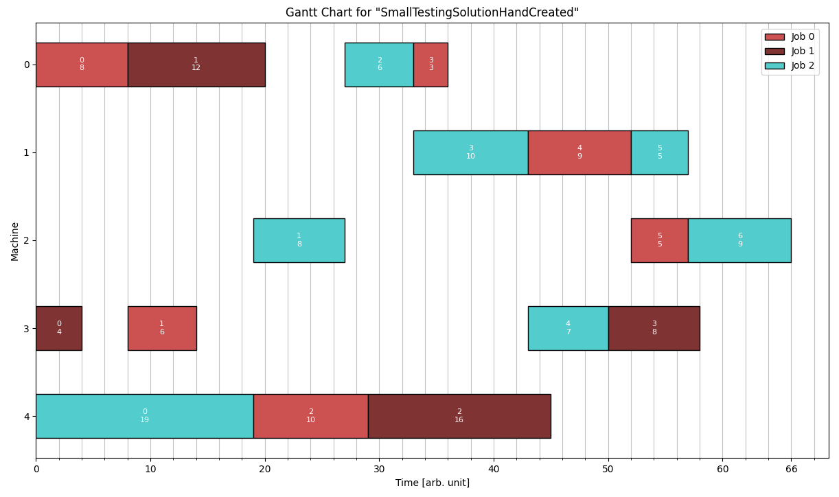
This is a Solution for the example problem given in the Detailed Format section.
# comments possible
SmallTestingSolutionHandCreated
3 5
4, 0 0 0 8 0 8, 1 1 0 12 8 20, 2 2 0 6 27 33, 0 3 0 3 33 36
3, 2 3 1 10 33 43, 0 4 1 9 43 52, 2 5 1 5 52 57
3, 2 1 2 8 19 27, 0 5 2 5 52 57, 2 6 2 9 57 66
4, 1 0 3 4 0 4, 0 1 3 6 8 14, 2 4 3 7 43 50, 1 3 3 8 50 58
3, 2 0 4 19 0 19, 0 2 4 10 19 29, 1 2 4 16 29 45
JobShopSolutions/SmallTestingSolution.txt
Using the Python Helper Script to create a Gantt Chart for this Solution gives:
A possible Solution for the abz5 problem shown in the Standard format section is:
Python Helper Scripts
The helper scripts are located in the 'PythonScripts' Folder at the root of the project. The two main scripts are "createGanttFromFile.py" and "Google_OR_Tools.py".
Create Gantt Visualization
Creates a visualization of a Solution using matplotlib. Example usage:
$ python createGanttFromFile.py -ri dmu/dmu06.txt
The only parameter is the path to a Solution file. The options allow relative paths to be used. Use the '-h' or '-help' flag to get the details about the available option flags.
For very large Solutions the chart may struggle to display all the labels in a readable manner.
Google OR Tools
This is a simple wrapper for the Google OR-Tools that can solve JobShop problems with a CP-Solver. It requires the installation of the ORTools module (see OR-Tools Install and follow the python guide).
The wrapper enforces a TIMEOUT constraint. Example usage:
$ python Google_OR_Tools.py -ri dmu/dmu06.txt -t 20
The script takes two parameters, the path to the Solution file and the timeout. Use the '-h' or '-help' flag to get the complete information about the usage.
Additionally there is also the 'runOR_Tools.py' script. It runs 'Google_OR_Tools.py' on multiple files.
'runOR_Tools.py' does not take any arguments, instead the code should be edited directly. Especially the python version must be set correctly as it currently uses an alias to a custom install location.
This script can only parse Problems in the Standard Format (you can convert between formats by loading the Problem with JS_Lib and the saving it in the desired format).